1. Why Elastic Net is Needed
Both regularization methods have advantages and limitations.
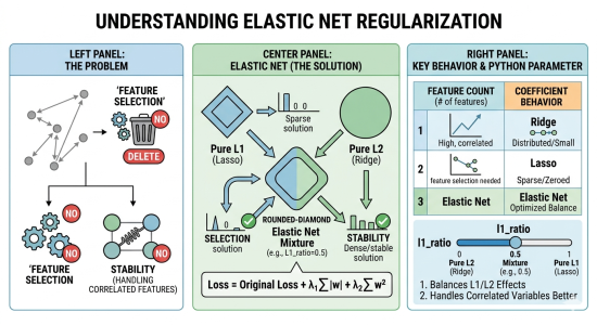
L1 regularization is particularly valuable because it performs automatic feature selection. By penalizing the absolute values of the weights, it can shrink some coefficients exactly to zero, effectively removing irrelevant features from the model. This property is extremely useful when dealing with high-dimensional data, as it produces sparse and interpretable models. However, L1 regularization becomes unstable when features are highly correlated. In such cases, it may arbitrarily select one feature while discarding others that contain similar information, leading to inconsistent models across different samples.
L2 regularization,` become exactly zero. As a result, all features remain in the model, but their influence is reduced. This produces smoother and more stable solutions, especially when predictors are correlated, because L2 tends to distribute importance across related features rather than selecting only one. The drawback, however, is that L2 does not perform feature selection; irrelevant variables may still remain in the model, potentially reducing interpretability and efficiency.
Elastic Net regularization addresses these issues by combining both penalties in a single objective function. It encourages sparsity like L1 while maintaining the stability of L2 in the presence of correlated predictors. Consequently, Elastic Net can select groups of related features together, avoid arbitrary exclusions, and produce models that are both interpretable and robust. For this reason, it is widely used in modern machine learning applications, particularly when dealing with high-dimensional datasets containing many correlated variables.
In short: both regularization methods have advantages and limitations.
L1 (Lasso)
- Performs feature selection
- Some weights become exactly zero
- But unstable when features are highly correlated
L2 (Ridge)
- Handles correlated features well
- Produces stable models
- But does not remove features
Elastic Net solves this by combining both penalties.
2. Elastic Net Loss Function
The loss function becomes:
\
Where:
- (Control L1 Strength): Controls the "Sparsity." As increases, more weights () are driven to exactly .
- (Control L2 Strength): Controls the "Smoothness." As increases, the weights are spread out more evenly, preventing any single feature from dominating.
So the model benefits from:
- feature selection (L1)
- stability (L2)
3. Intuition
So the model benefits from:
- feature selection (L1)
- stability (L2)
So the model is both sparse and stable.
from sklearn.linear_model import LogisticRegression
import numpy as np

X = np.array([[1],[2],[3],[4],[5]])
y = np.array([0,0,0,1,1])

model = LogisticRegression(
    penalty='elasticnet',
    solver='saga',
    l1_ratio=0.5
)

model.fit(X,y)

print("Weights:", model.coef_)
print("Bias:", model.intercept_)
Important parameter: l1_ratio
| Value | Meaning |
|---|---|
| 0 | pure L2 |
| 1 | pure L1 |
| 0.5 | mixture |
Solvers:
A solver is the method that finds optimal weights by minimising loss. Different datasets require different strategies:
- Small datasets, Large datasets
- High-dimensional data
- L1, L2 or Elastic net
-
lbfgs solver: The lbfgs solver is the industry standard and the default in many libraries because it is fast, stable, and handles the majority of general-purpose problems efficiently, provided you only require L2 regularization.
- liblinear solver: For smaller datasets where you might need feature selection through L1 regularization, The liblinear is a robust choice that handles both L1 and L2 penalties effectively.
- saga solver: It serves as its more versatile evolution; it is the only solver that supports L1, L2, and Elastic Net regularization while maintaining high performance on large datasets.
- sag solver: When dealing with large-scale data, the Stochastic Average Gradient descent variants are more appropriate. While sag is highly efficient for massive datasets using L2 regularization.
Comparison table of the Solver
| Solver | Regularization | Best For... | Multiclass Support | Key Note |
| lbfgs | L2, None | General cases & medium datasets | Multinomial (Direct) | Default in Scikit-Learn; memory-efficient and stable. |
| liblinear | L1, L2 | Small datasets & sparse data | One-vs-Rest (OvR) only | Cannot do true multinomial loss; good for high-dimensional binary problems. |
| saga | L1, L2, Elastic Net | Very large datasets | Multinomial (Direct) | An extension of SAG that supports L1; the most versatile solver. |
| sag | L2, None | Large datasets | Multinomial (Direct) | Fast convergence but requires all features to be on a similar scale. |
3. When to Use Elastic Net
Elastic Net is commonly used when:
- Dataset has many features
- Features are correlated
- Want automatic feature selection
Examples:
- Finance prediction
- Medical data
- Text classification