1. Training Logistic Regression
In logistic regression, the goal is to learn the optimal weights and bias so that the predicted probabilities are as close as possible to the true labels.
This is achieved by minimizing the Binary Cross-Entropy loss function using an optimization algorithm such as gradient descent.
Training involves three main steps:
- Compute predicted probabilities using the sigmoid function.
- Compute the loss using the cross-entropy formula.
- Update the model parameters (weights and bias) to reduce the loss.
2. Gradient Descent Optimization
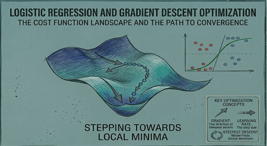
Gradient descent is an iterative optimization algorithm used to minimize the loss function. At each iteration, the parameters are updated in the direction that reduces the loss.
Parameter Update Rules
This formula represents the Gradient Descent update rule, which is the "engine" that allows machine learning models to learn by iteratively adjusting their weights.
Weights:
Bias:
key point: The gradients measure how much the loss changes when the parameters change.
| Symbol | Meaning |
|---|---|
| () | weight of feature (j) |
| (b) | bias |
| (L) | loss function |
| (\alpha) | learning rate |
3. Gradient of Logistic Regression
For logistic regression, the gradients are:
Weight Gradient
Bias Gradient
| Symbol | Meaning |
|---|---|
| () | true label |
| () | predicted probability |
| () | feature value |
| (n) | number of samples |
4. Applying Gradient Computation to Our Example
| Sample | True Label (y) | Predicted Probability (p) |
|---|---|---|
| 1 | 1 | 0.9 |
| 2 | 0 | 0.2 |
Step 1: Compute Prediction Error
To render the error (or residual), which represents the difference between your model's prediction and the actual target, use the following equation:
| Sample | (y) | (p) | Error |
|---|---|---|---|
| 1 | 1 | 0.9 | -0.1 |
| 2 | 0 | 0.2 | 0.2 |
Step 2: Compute Bias Gradient
So
5. Parameter Update Example
Assume
Initial bias b = 0
Learning rate
Update rule
Substitute values
Thus the bias decreases slightly to reduce the loss.
6. Summary Iterative Learning Process
The goal of training is to find parameters w and b that minimize the average log loss:
Training logistic regression involves repeating the following steps:
The mathematics behind your logistic regression program, step by step
import numpy as np
import matplotlib.pyplot as plt
from sklearn.linear_model import LogisticRegression

# Sample dataset
X = np.array([[1], [2], [3], [4], [5]])
y = np.array([0, 0, 0, 1, 1])

# Model
model = LogisticRegression()
model.fit(X, y)

# Predictions for curve
X_test = np.linspace(0, 6, 100).reshape(-1, 1)
y_prob = model.predict_proba(X_test)[:, 1]

# Decision boundary (where probability = 0.5)
decision_boundary = X_test[np.argmin(np.abs(y_prob - 0.5))][0]

# Plot
plt.figure(figsize=(8,5))
plt.scatter(X, y, color='blue', label='Data points')
plt.plot(X_test, y_prob, color='red', label='Sigmoid curve')
plt.axvline(x=decision_boundary, color='green', linestyle='--', label=f'Decision Boundary ≈ {decision_boundary:.2f}')
plt.xlabel("Feature")
plt.ylabel("Probability / Class")
plt.title("Logistic Regression Curve with Decision Boundary")
plt.legend()
plt.show()
The Dataset:
Where:
For a single feature, .
- w = weight (learned by model)
- b = bias (learned by model)
- σ(z) = sigmoid function
The sigmoid function maps any real number to a probability (0–1):
-
As : The term (which is ) approaches 0. Thus, the denominator becomes , and the entire fraction .
-
As : The term grows infinitely large. When the denominator of a fraction becomes infinitely large, the value of the fraction .
-
At : . This is typically the "neutral" point or decision boundary.
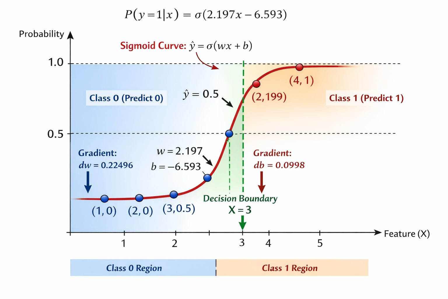
Assume after fitting your model.fit(X, y), sklearn gives:
w≈2.197, b≈−6.593
(These values come from fitting a simple logistic regression on this small dataset.)
Now calculate probability for each X:
| X | z = w*X+b | sigmoid(z) = 1 / (1+e^-z) |
|---|---|---|
| 1 | 2.197*1 -6.593 = -4.396 | σ(-4.396) ≈ 0.012 |
| 2 | 2.197*2 -6.593 = -2.199 | σ(-2.199) ≈ 0.100 |
| 3 | 2.197*3 -6.593 = -0.002 | σ(-0.002) ≈ 0.500 |
| 4 | 2.197*4 -6.593 = 2.195 | σ(2.195) ≈ 0.899 |
| 5 | 2.197*5 -6.593 = 4.392 | σ(4.392) ≈ 0.988 |
Notice how probabilities rise from 0 → 1 as X increases..
This ensures our outputs are valid probabilities.
y_prob = model.predict_proba(X_test)[:, 1]This calculates for each value in X_test.
Loss Function (Cross-Entropy / Log Loss)
To learn w and b, logistic regression minimizes the log loss:
Where:
-
- n = number of samples
Plugging in numbers:
- i=1: y=0, ŷ=0.012 → −[0∗log(0.012)+(1−0)∗log(1−0.012)]=−log(0.988)≈0.012
- i=2: y=0, ŷ=0.100 → -log(0.900) ≈ 0.105
- i=3: y=0, ŷ=0.500 → -log(0.500) ≈ 0.693
- i=4: y=1, ŷ=0.899 → -log(0.899) ≈ 0.106
- i=5: y=1, ŷ=0.988 → -log(0.988) ≈ 0.012
Average loss:
This penalises predictions far from the true label.
Optimization (Gradient Descent)
Scikit-learn uses iterative optimization (like gradient descent) to minimize J(w,b).
The gradients are:
Once you calculate this gradient, you update the weight using a Learning Rate ():
This is done internally by model.fit(X, y).
Compute each term:
- ŷ - y for each i:
| X | y | ŷ | ŷ - y |
|---|---|---|---|
| 1 | 0 | 0.012 | 0.012 |
| 2 | 0 | 0.100 | 0.100 |
| 3 | 0 | 0.500 | 0.500 |
| 4 | 1 | 0.899 | -0.101 |
| 5 | 1 | 0.988 | -0.012 |
- Multiply by X for dw:
| X | ŷ - y | (ŷ - y)*X |
|---|---|---|
| 1 | 0.012 | 0.012 |
| 2 | 0.100 | 0.200 |
| 3 | 0.500 | 1.500 |
| 4 | -0.101 | -0.404 |
| 5 | -0.012 | -0.060 |
Sum: 0.012+0.200+1.500-0.404-0.060 ≈ 1.248
Divide by n=5 → dw ≈ 0.2496
For db:
Sum of (ŷ-y): 0.012+0.100+0.500-0.101-0.012 ≈ 0.499
Divide by n=5 → db ≈ 0.0998
Weight Update (One Step)
Assume learning rate α = 0.1:
w:=w−α⋅dw=2.197−0.1∗0.2496≈2.172
b:=b−α⋅db=−6.593−0.1∗0.0998≈−6.603
This step moves weights toward minimising loss. This step moves weights toward minimizing loss.
Decision Boundary
The decision boundary is where the predicted probability = 0.5: σ ( w⋅x + b )=0.5
Solve for x: