1. Introduction
Logistic Regression is a classification algorithm used to predict the probability that a sample belongs to a class. Unlike linear regression, which predicts continuous values, logistic regression predicts probabilities between 0 and 1, making it suitable for binary classification problems.
Applications
- Email spam detection
- Disease diagnosis (e.g., diabetes prediction)
- Student pass/fail prediction
- Customer churn prediction
2. Linear vs Logistic Regression
| Feature | Linear Regression | Logistic Regression |
|---|---|---|
| Output | Any real number | Probability (0–1) |
| Problem Type | Regression | Classification |
| Loss Function | MSE | Binary Cross-Entropy |
| Activation | None | Sigmoid |
3. Sigmoid Function in Logistic Regression
The sigmoid function is the mathematical function used in logistic regression to convert any real-valued number into a probability between 0 and 1 (see Figure 1).
Figure 1. Sigmoid function
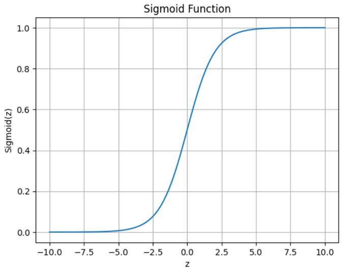
- Converts the linear combination of features into a probability.
- Output ranges between 0 (class 0) and 1 (class 1).
The sigmoid function is defined as:
Alternatively,
where:
or
or in vector form
Components:
 = input features
 = weights
 = bias
 = linear combination
 = Euler’s constant
4. Logistic Regression Model
The logistic regression model first computes a linear combination of features, then applies the sigmoid function.
Linear Model:
Probability Model
Figure 2. Logistic Function
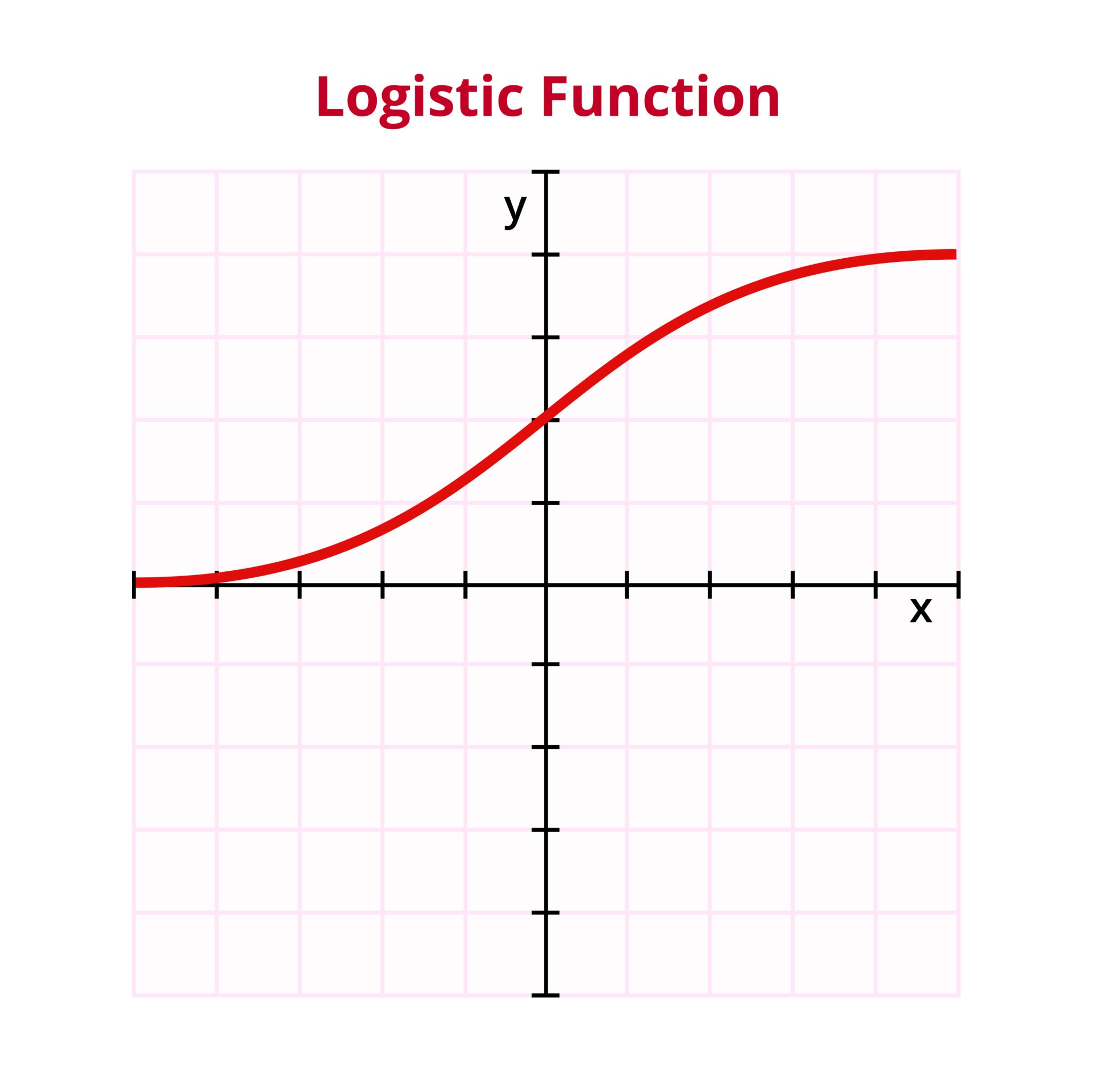
Exponent: The exponent ensures that no matter how large or small the value of z becomes, the output remains a valid probability between 0 and 1.
Decision Rule
The predicted class is determined using a threshold of 0.5.
Decision Boundary
The decision boundary occurs when the predicted probability equals 0.5.
Since, Sigmoid function is:
Substitute in sigmoid:
| Step | Rendered Result |
| 1. Reciprocal | |
| 2. Simplify | |
| 3. Isolate | |
| 4. Natural Log | |
| 5. Final |
this implies:
Therefore the decision boundary condition is:
Solving for x:
For:
- 1 feature → point, e.g., for x:
- 2 features → line e.g., , for x2:
- 3 features → plane
- n features → hyperplane
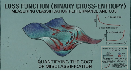
5. Loss Function (Binary Cross-Entropy)
The Binary Cross-Entropy Loss (also known as Log Loss) is the standard cost function used to train logistic regression.
- Measures prediction error
- Smaller loss → better model
- Works well with probabilities instead of hard labels
Example Table:
| Sample | Actual Label (y) | Predicted P ( y = 1) | Loss |
| 1 | 1 | 0.9 | 0.105 |
| 2 | 0 | 0.2 | 0.223 |
For a single sample:
Where
- y= true label
- p = predicted probability P(y=1)
| Actual Label | Predicted Label |
| y=1 | p = 0.9 |
Calculation for Sample 1
Step 1: Substitute values
Step 2: Simplify
Step 3: Compute log
Step 4: Final loss
Loss = 0.105
Calculation for Sample 2
Step 1: Substitute values
Step 2: Simplify
Step 3: Compute log
Step 4: Final loss
Loss = 0.223
| Sample | True Label (y) | Predicted (p) | Loss (L) |
| 1 | 1 | 0.9 | 0.105 |
| 2 | 0 | 0.2 | 0.223 |
4. Average Loss for the Dataset
If we average the losses from both samples:
5. Interpretation
Log Loss penalizes the model based on how far the predicted probability is from the true label.
Example Analysis:
Sample 1:
for
This is a strong and correct prediction, producing a small loss (0.105).
Sample 2:
for
This is also a correct prediction, but with slightly less confidence, producing a larger loss (0.223).
Key Note: During training, the goal is to minimize the average loss across all samples, pushing predicted probabilities closer to the true labels..