1. Introduction
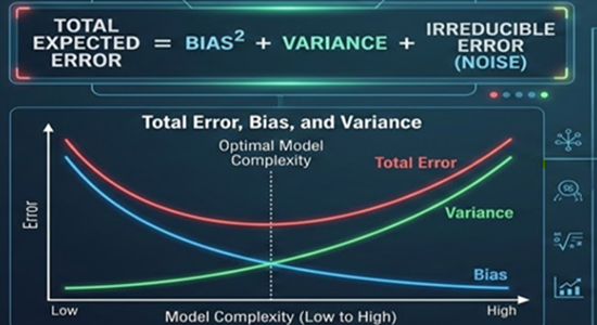
When training models in machine learning, we want the model to learn patterns from the training data and make accurate predictions on unseen data. On the other hand, the expected prediction error in machine learning is decomposed into three parts known as 'predictive error decomposition' or 'total prediction error of a model', which can be decomposed as
Where:
: Error caused by incorrect assumptions in the model.
Variance: Error caused by sensitivity to fluctuations in the training data.
Irreducible Error: Noise inherent in the data that cannot be eliminated.
Example sources:
- measurement noise
- randomness in observations
- incomplete features
Error ≠ Bias :Bias is only one contributor to the total error.
2. What Bias and Variance Represents
In Machine Learning, the Bias–Variance concept explains why models make errors and how model complexity affects performance.
2.1. Bias
Bias measures how far the model's average prediction is from the true function.
Where:
: True function
: Expected prediction
: Predicted Model
Squared Bias:
Characteristics of Bias
High Bias Model:
- Oversimplified
- Cannot capture patterns
- Underfitting
Examples:
- Linear regression for nonlinear data
- Very shallow neural network
Key point: the goal of the ML engineer should be to obtained low bias model.
For example, suppose the true relationship is the following:
And the training data:
| x | True y |
|---|---|
| 1 | 1 |
| 2 | 4 |
| 3 | 9 |
If the model assumes:
Predictions may be:
| x | True y | Predicted |
|---|---|---|
| 1 | 1 | 2 |
| 2 | 4 | 3 |
| 3 | 9 | 4 |
Let's estimate the bias average prediction error for the above model:
| x | True y | Predicted | Error ((\hat{y}-y)) |
|---|---|---|---|
| 1 | 1 | 2 | 1 |
| 2 | 4 | 3 | -1 |
| 3 | 9 | 4 | -5 |
Bias = −1.67
Interpretation
Bias = -1.67
Meaning:
- The model predictions are on average 1.67 units lower than the true values.
- This indicates systematic error, hence high bias (underfitting).
The model cannot capture the quadratic relationship because it is likely a simple linear model.
2.2. Variance
Variance measures how much predictions change when training data changes.
Where:
- : Prediction from a particular training dataset
- : Average prediction over many datasets
Characteristics of variance
High Variance Model:
- Very complex
- Fits training data closely
- Overfitting
Examples:
- Deep decision tree
- High-degree polynomial
- Very complex neural networks
Example:
Training datasets:
Dataset 1 → Model predicts: 5
Dataset 2 → Model predicts: 9
Dataset 3 → Model predicts: 2
Average prediction:
Variance:
=8.21 (A large value means high variance.)
2.3. What Irreducible Error Means
Even if we had the perfect model, there is still noise in data. Example: house price prediction where two identical houses may sell for different prices due to the following:
- negotiation
- market conditions
- random factors
This randomness cannot be removed. This is irreducible error.
3. Bias², Variance, and MSE
Let's compute Bias², Variance, and MSE together using a simple numerical example. This is the standard demonstration used in machine learning courses.
3.1. Problem Setup
Suppose the true value of the function at x is:
We train the model on different datasets, producing different predictions. where total number of models are (n=4)
| Model | Prediction |
|---|---|
| Model 1 | 8 |
| Model 2 | 9 |
| Model 3 | 12 |
| Model 4 | 11 |
Step 1: Average Prediction
E[\hat{f}(x)] = 10
Step 2: Compute Bias
Bias=0
Step 3: Bias²
Interpretation:
- The average model prediction is exactly correct
- The model has no systematic error
Step 4: Variance
| Prediction | Deviation from mean | Squared |
|---|---|---|
| 8 | 8−10 = −2 | 4 |
| 9 | 9−10 = −1 | 1 |
| 12 | 12−10 = 2 | 4 |
| 11 | 11−10 = 1 | 1 |
\text{Var} = \frac{10}{4} = 2.5
Step 5: Mean Squared Error (MSE)
\text{MSE} = \frac{1}{n} \sum (\hat{f}_i - f(x))^2
| Prediction | True value | Error | Error² |
|---|---|---|---|
| 8 | 10 | -2 | 4 |
| 9 | 10 | -1 | 1 |
| 12 | 10 | 2 | 4 |
| 11 | 10 | 1 | 1 |
3.1. Verify Bias–Variance Decomposition
MSE=0+2.5
MSE=2.5
Interpretation
| Component | Value | Meaning |
|---|---|---|
| Bias² | 0 | No systematic error |
| Variance | 2.5 | Predictions fluctuate |
| MSE | 2.5 | Total prediction error |
- The model is unbiased
- But predictions vary due to variance.
Conclusion:
Think of three model types:
| Model Type | Bias | Variance |
|---|---|---|
| Underfitting | High | Low |
| Optimal | Low | Low |
| Overfitting | Low | High |